Fundamentals of Algorithm Design: Sorting, Searching & Algorithmic Complexity

Algorithm design programming represents the foundational computational discipline of software engineering. An algorithm is an unambiguous, finite sequence of rigorous instructions engineered to solve a specific mathematical or computational problem. Whether indexing billions of web pages, optimizing supply chain routes, or processing real-time graphics, algorithmic efficiency determines whether a software application scales smoothly or crashes under enterprise loads.

1. Core Attributes of an Efficient Algorithm

To be mathematically valid and practically viable in production, an algorithm must satisfy five foundational criteria:

• Unambiguous & Clear: Every instructional step must be mathematically precise, leaving zero ambiguity in execution logic.
• Defined Inputs & Outputs: Accepts zero or more well-defined inputs and deterministically yields specified outputs.
• Finiteness: The execution path must reliably terminate after a finite number of steps across all valid input conditions.
• Feasibility: The process must be computationally practical using available memory and processor cycles.
• Language Agnostic: The algorithmic logic should be expressible in plain language, mathematical notation, flowcharts, or pseudocode, independent of specific programming languages.

2. Foundational Sorting Algorithms: Bubble Sort in Detail

Sorting unordered datasets is one of the most fundamental operations in computer science. Bubble Sort is the classic introductory comparison sort:

• Mechanism: Iterates repeatedly through an array, comparing adjacent elements and swapping them if they are in the wrong order. With each complete pass, the largest remaining element “bubbles up” to its final position at the end of the list.
• Algorithmic Pseudocode:

procedure BubbleSort(A : list of sortable items)
    n = length(A)
    repeat
        swapped = false
        for i = 1 to n-1 inclusive do
            if A[i-1] > A[i] then
                swap(A[i-1], A[i])
                swapped = true
            end if
        end for
        n = n - 1
    until not swapped
end procedure

• Complexity Analysis: While simple to understand and implement in memory ($O(1)$ auxiliary space), Bubble Sort exhibits quadratic time complexity ($O(n^2)$), rendering it impractical for production datasets where advanced divide-and-conquer algorithms (QuickSort, MergeSort) are preferred.

3. Search Paradigms: Linear Search vs. Binary Search

Locating a target value within an array represents another ubiquitous programming challenge:

• Linear Search: Inspects every element sequentially from the first index to the last until a match is found. While it functions on unsorted arrays, its time complexity scales linearly ($O(n)$).
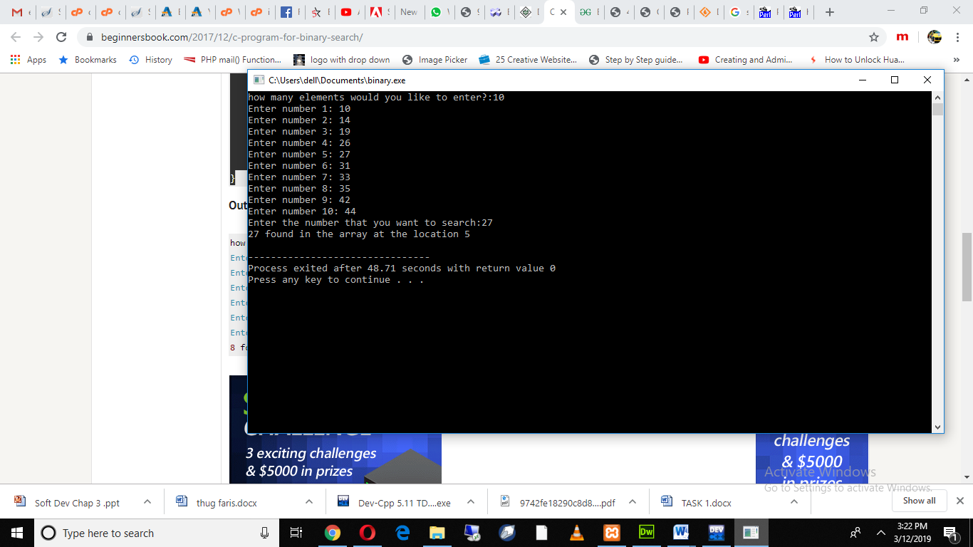
• Binary Search: Operates on pre-sorted arrays by repeatedly dividing the search space in half. By comparing the target value to the middle element, it eliminates half the remaining elements in each step, achieving exceptional logarithmic time efficiency ($O(log n)$).

4. Big O Notation: Evaluating Time and Space Complexity

Engineers analyze algorithmic efficiency using Big O Notation, which models the upper bound of resource consumption as input size ($n$) scales toward infinity:

Frequently Asked Questions (FAQ)

Why is Big O notation focused on the worst-case scenario?

Worst-case analysis guarantees that an algorithm will never exceed a specific time or memory boundary, providing reliable performance guarantees for mission-critical software systems.

When should Binary Search be used over Linear Search?

Binary Search should always be used on large datasets when the data is already sorted (or when search queries are frequent enough to justify the initial cost of sorting the array).

What is the difference between time complexity and space complexity?

Time complexity measures the number of computational operations an algorithm executes as input size grows. Space complexity measures the amount of working memory (RAM) the algorithm allocates during execution.

Conclusion

Proficiency in algorithm design programming separates skilled software engineers from casual coders. By mastering core sorting and searching paradigms and applying Big O complexity analysis, developers write clean, high-performance code that scales effortlessly to meet modern enterprise demands.

def quicksort_median_of_three(arr, low, high):
    """
    Guarantees O(n log n) average time complexity by mitigating O(n^2) worst-case 
    degeneracy on sorted or reverse-sorted input arrays.
    """
    if low < high:
        pivot_idx = partition(arr, low, high)
        quicksort_median_of_three(arr, low, pivot_idx - 1)
        quicksort_median_of_three(arr, pivot_idx + 1, high)

def partition(arr, low, high):
    mid = (low + high) // 2
    # Sort low, mid, high elements to select median
    if arr[low] > arr[mid]: arr[low], arr[mid] = arr[mid], arr[low]
    if arr[low] > arr[high]: arr[low], arr[high] = arr[high], arr[low]
    if arr[mid] > arr[high]: arr[mid], arr[high] = arr[high], arr[mid]
    
    # Place median at high - 1 as pivot
    arr[mid], arr[high] = arr[high], arr[mid]
    pivot = arr[high]
    i = low - 1
    for j in range(low, high):
        if arr[j] <= pivot:
            i += 1
            arr[i], arr[j] = arr[j], arr[i]
    arr[i + 1], arr[high] = arr[high], arr[i + 1]
    return i + 1